Questions:
Why is the analysis focused on only the 20th century?
At the time of analysis, for instrumental data, complete time series for indices that constitute a spatially representative climate network were available for only the 20th century.
What methodology was used?
Multi-channel Singular Spectrum Analysis (MSSA). Discussion of this method continues in various paragraphs below.
What is the periodicity of the stadium wave?
This is not determinable. This is because the shared variability among indices in the climate network occurs on a multi-decadal timescale (~64 years peak-to-peak in 20th century). The index time series are only 100 years long. To be eligible for qualifying as a statistically significant signal, the signal's periodicity must be well within a window size ~1/5 the length of a time series. For a century's worth of data, that requires a periodicity of less than or equal to 20 years.
The method (Multi-channel Singular Spectrum Analysis (MSSA)) used in the stadium-wave studies could have identified a statistically significant signal with a period of 20 years or less, if, indeed, all indices in the stadium-wave network possessed this signal. They did not. But beyond identifying shorter-term periodicities, MSSA also can identify trends that fall outside this shorter timescale, but only if that trend is shared by all network indices. As established, assigning statistical significance to a trend of that time scale is not possible. This was the case for the stadium wave. A low-frequency signal shared by all network indices was identified, but its periodicity was not eligible for statistical-significance testing. Therefore, we frame the stadium wave thusly: it is a secularly varying trend that oscillates with apparent regularity; although not at a defined periodicity. The term 'secular' refers to a long-term timescale.
Worth mention is the observation that even though all network indices share the identified stadium-wave signal, the fraction (%) of each index's variance that was accounted for by the stadium-wave signal differs according to index. The stadium-wave signal accounts for a substantial fraction of index variance in ocean indices, ice indices in the Western Eurasian Arctic seas, surface Arctic and Northern Hemisphere temperatures, and large-scale wind-flow patterns. Wintertime atmospheric circulation patterns, such as the North Atlantic Oscillation, and the oceanic-atmospheric pattern of El Nino-Southern Oscillation are dominated by high-frequency behavior. Thus, the variance in these two indices accounted for by the stadium-wave signal is low (see Figure 5 in Wyatt and Curry2013).
If periodicity cannot be determined, how can the signal be statistically significant at the 95% confidence level?
While the periodicity of the signal cannot be assigned statistical significance (due to short time series and long timescale of variability), the alignment of indices all possessing this low-frequency signal can be. And it is robustly statistically significant. For the original eight-member network (Wyatt, Kravtsov, and Tsonis 2012 (WKT)), the alignment was significant at p<3%, or the 97% confidence level. For the expanded 15-member network (Wyatt and Curry 2013 (WC)), the significance was p<5%, or 95% confidence level.
What does 'alignment of indices' mean and how was its statistical significance ascertained?
Alignment is what defines the propagation sequence of the stadium wave. Propagation is the essence of this signal. In this research, we asked, "What are the chances that a shared low-frequency alignment of regionally and dynamically diverse indices could occur just by random chance?" To quantify an answer to this question, we used a red-noise numerical model (WKT; WC) to randomly generate time-series values. We then applied MSSA to those 'fake' or uncorrelated, random-valued index time series. We treated the uncorrelated indices in the same manner as we had the 'real' index time series. We did this many times with the red-noise-model-generated data (100 in WKT and 1000 in WC). In less than 3% of the cases in WKT, and less than 5% of the cases for WC, those uncorrelated ('fake') indices showed low-frequency alignment (i.e. consistent sequence of propagation). This is the statistical outcome one desires to nullify the hypothesis that states the signal is due to random occurrence, as that occurrence was found to be less than 3% (in WKT) and 5% ( in WC). Thus, it can be fairly concluded that the propagation sequence and timescale of variability characterizing the stadium wave is not merely the result of random red-noise. The possibility that the stadium-wave's low-frequency alignment is only a random artifact of uncorrelated red-noise in the data is extremely low.
The plots of the stadium wave look like a bunch of sine curves. The data appear to be heavily filtered. How credible are these results?
Again, the "results" of the stadium wave make no claims regarding periodicity; instead, the results involve the low-frequency alignment that is found unlikely to be due to random occurrence at a confidence level of at least 95% (or p < 5%) for all spatially representative index networks. That the data appear to be 'heavily filtered' and a 'bunch of sine curves' is a function of a couple of things.
First, the data are filtered, but not in a way one might assume. The filter is not 'pre-prescribed'; rather, it is data-adaptive. And unlike a filtering method such as box-car type low-pass filtering, the phase error (where the peaks and troughs occur), while not completely eliminated, is much less pronounced. MSSA is essentially the same as Empirical Orthogonal Analysis (EOF analysis). The major difference between the two is that EOF analysis seeks correlations of indices at a zero-lag; whereas MSSA identifies correlations of indices at both zero and non-zero lags.
To execute the MSSA methodology, time series of raw data are put in channels of a lagged co-variance matrix. Each index-channel is repeated in the matrix twenty times at a one-year lag. This means there are 20 copies of each index. The lags in alignment allow for identification of lagged co-variance (propagation). The 20 copies represent a filter, M=20 years, that is used to identify any shared index periodicity, or oscillation, of 20 years or less. As mentioned previously, such higher-frequency periodicities shared by all network indices were not found. For 'trends' with a timescale of variability greater than the imposed window of 20 years (in this case), the timescales of variability shared by all indices in the lagged co-variance matrix become the 'filter'. MSSA isolates the modes, or patterns, of co-variability and filters all others out. Indices of all the spatially representative climate network combinations showed shared variability at an approximate 60-year timescale (for 20th century). Results showed that all indices co-varied with two modes. Both modes oscillated at the same secular timescale. Combining these two modes yielded the 'filtered signal'.
Critical to the effectiveness of MSSA, and necessary for avoiding over-fitting, data must be spatially representative. If too many indices come from just one small geographical region, one risks inserting a bias into the data-adaptive filter. Thus, not only do we seek greater temporal representation; we seek greater spatial representation, as well. And we achieve that with indices from the low, mid, and high latitudes, and from various longitudes within, over, and adjacent to the North Atlantic, North Pacific, the Arctic, and Eurasia. Further augmenting the spatial representation of the stadium-wave network could be done by adding indices from the Indian Ocean and from the Southern Ocean, for examples. Data availability can be the limiting factor.
What about red-noise contamination?
Geophysical time series typically are characterized by the presence of noise with substantial power in the low-frequency portion of the spectrum. This is known as red-noise and is due to 'memory', or persistence of signal, in these geophysical systems. Inertia of slowly varying factors - e.g. sea-surface temperatures, soil moisture, polar ice, snow cover, and the like - leave vestiges in the system that carry over into the next year, or two, or more; this being the source of memory and of spurious 'cycles' that can emerge in a time series. Even if no real cyclic behavior existed, a time series contaminated with red-noise could still exhibit cycles. Thus, in a time series characterized by true cycles, the additional red-noise-related 'cycles' may mask or distort expression of the real periodic or quasi-periodic cycles.
Pure temporal filtering (e.g. low-pass) of a mixture of quasi-periodic time series containing a strong red-noise component may erroneously reflect this low-frequency variability. Adding a spatial component to the filter lessens this likelihood. MSSA has the spatial component. The matrix of time series that is the stadium-wave network represents spatial diversity. Indices derive from across a broad (hemispheric) geographical area. Thus, if a quasi-periodic signal is characterized by a spatial structure that is distinct from the red-noise component, i.e. a 'real' signal, separation of signal from the noise using the spatio-temporal filter of MSSA is more robust. This highlights the advantage of MSSA over purely temporal methods of filtering.
What were the results of the spatio-temporal filtering and how is it done?
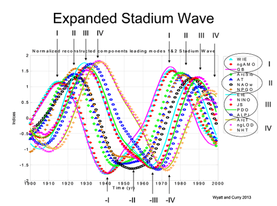
Two leading modes - i.e. dominant patterns of variability - were identified, each with a quasi-periodic signature of about 60 to 65 years.
To identify these modes, MSSA was applied to the extended (lagged copies) matrix of indices. The method identifies the patterns of variability shared among all the indices. We considered the mean variances of the first ten. The modes that were identified accounted for varying degrees of index behavior. A plot of the mean variance of each mode for the stadium-wave network showed the two leading modes to be well separated from the remaining modes. They were tested for statistical significance, and determined to be robust (p < 5%; discussed previously).
How are these modes represented in the stadium-wave signal?
They are represented on plots by reconstructed components. Reconstructed components, or RCs, are effectively the narrow-band filtered version of an original index time series. They are related to the coefficients (or EOF weights) of MSSA decomposition of the collection of time series under consideration. RCs are analogous to principal components (PCs) generated in EOF analysis. Yet, there is a difference. PCs are mutually orthogonal. RCs are not. Instead, the sum of all MSSA modes as represented by RCs, is identical to the original time series.
RCs were generated and plotted for each of the ten modes considered. The leading two modes, as identified by the plotted mean variances (see previous section), each reflected a quasi-periodicity of ~60 to 65 years. RCs of leading modes one and two were combined. This created the stadium-wave signal, or its associated filter. RCs of the combined two leading modes are what one sees representing each index on the stadium-wave plots. The time series of the RCs are normalized to unit variance for ease of comparison.
Were the non-leading modes of variability considered?
Yes. But not the individual modes, rather the collection of modes. This 'residual' information -- information isolated from the two leading modes -- was analyzed. Inter-annual to inter-decadal variability dominated its behavior. In WKT, correlations among the high-frequency indices were identified. At specific times over the century, correlations between indices in the collection were strong. Three of the episodes of strong correlations occurred at times of 20th-century multi-decadal regime shifts. Approximate dates for these include: ~1918, 1942, and 1976. WKT speculated on the result. These dates reflect similar results from Tsonis et al (2007) and Swanson and Tsonis (2009), where episodes occurring at these times were described as 'successful synchronizations'. These successful synchronizations coincide with multi-decadal regime shifts as identified in WKT and WC. WKT and WC found that climate-regime shifts are characterized by a reversal in trend of the AMO (Atlantic Multi-decadal Oscillation) anomalies; while the polarity of PDO (Pacific Decadal Oscillation) anomalies reverses simultaneously, or nearly so. [Warm regime: increasing trend of AMO w/ positive PDO; Cool regime: decreasing trend of AMO w/ negative PDO.] Such regime-shifts coincide with peaks and troughs in indices of 'group I', as identified in WC.
In addition, Tsonis et al. and Swanson and Tsonis had identified unsuccessful synchronizations occurring in ~1923 and 1957. WKT results also identified these episodes of strong correlations within the residual data set. In addition, WKT also showed correlations in the early-mid 1980s. These three dates, 1923, 1957, and early-mid-1980s, coincide with trend reversals in the plots of 'group II' in WC. The reason for this is unclear, but invites further study. According to WC, this timing reflects the transformation of an Atlantic-oceanic signal into an oppositely signed atmospheric one (see stadium-wave description on previous web page). WKT also identified one other strong correlation occurring in the 20th century -- in the late 1990s.
Can you be sure this signal is not contaminated or influenced by anthropogenic emissions of greenhouse gases?
No. We cannot claim certainty about that. When we ran our MSSA program, we linearly detrended the data. MSSA requires that the mean of each index be removed before testing for index co-variability. We chose to linearly detrend, which leaves a mean of zero for each index. We linearly detrended in order to satisfy the requirement that the mean=0, and, as an additional purpose, in order to highlight multi-decadal variability. We could speculate that this operation removed a significant portion of the anthropogenic fingerprint, but likely not all. Thus, not knowing with certainty if the anthropogenic signal was fully removed, it could be fairly argued that anthropogenic emissions have contaminated the stadium-wave signal. There may be ways to check this (see Kravtsov and Spanngle (2008)). But an indirect argument can be found in the use of proxy data. In my dissertation research (Wyatt 2012), I tested a variety of proxy data for the 20th century. Using the proxy-index collections that generated a statistically significant low-frequency alignment identical to the instrumental-data version, I carried analysis back to 1700. Results showed that propagation alignment remains unchanged, but amplitude and frequency of wave propagation modified prior to ~1800. How much those features modified depended on which proxies were used. Now, the observed changes could be from the errors (noise) inherent in proxy data, or it could be from a real behavior change. This can't be known for certain. But the fact that the character of the stadium-wave signal appears to be unchanged throughout a time period (at least since 1850) over which CO2 levels have been increasing suggests that greenhouse-gas forcing has had little, if any, effect on this multi-decadal component. The observed pre-1800 change-in-character exhibited by the stadium wave appears to be more consistent with changes in solar irradiance rather than with changes in greenhouse-gas emissions. This is an on-going topic of research.
How might changes in solar output affect the stadium wave?
The speculative short answer is that it does two things: one, it provides the basic energy needed for oscillatory behavior, and appears to moderate amplitude of the hypothesized stadium-wave (e.g. between 1700 and 1800); and two, it entrains the frequency of the network rhythm.
The former influence is self-explanatory. The latter is less so; although it is a common dynamic. You may notice it when you are dancing or walking with someone arm-in-arm. You and your partner move with matched rhythm; your movements are 'synchronized'. Hasten the beat of the music, and your synchronized tempo increases too, synchronizing to the external pace. If the change of the music's tempo is strongly mis-matched to yours, it has no impact on the rhythm of you and your dance partner. You do not synchronize to it. In a like manner, a synchronized network's natural rhythm can be modified via weak coupling with an external forcing whose oscillatory tempo is similar to that of the synchronized network.
Solar output varies on many timescales - approximately at an average of 11 years, 22 years, 50 to 90 years, 200 years, and longer. The amount of variable output is relatively low; thus, direct forcing of climate on these timescales is small. Thus, it may be that the 50-to-90-year 'cycle' (Gleissberg) couples with the climate network and nudges the network's collective cadence. But how does this 'beat' couple with the network? What feature or features does the solar component entrain? The oceans, with their long memories and therefore long timescales of variability, appear likely candidates. In fact, paleoclimate evidence suggests correlation between solar output and low-frequency signals in the North Atlantic (e.g. Black et al. 1999; Bond et al. 2001). But still, the question is how.
Theories on indirect climate forcing abound, with different mechanisms involving differences in latitudes, longitudes, altitudes, and dynamics of forcing proffered: changes in sea-level-pressure of major centers-of-action (e.g. Georgieva et al. 2007; VanLoon et al. 2007); changes in ocean-heat-content in the tropics via stratosphere-down dynamics (e.g. White 2006); changes in cloud cover due to changes in solar wind and its modulation of incoming galactic cosmic radiation (e.g. Svensmark and Friis-Christensen 1997); changes in ozone levels in the polar vortex (Shindell et al. 1999); changes in electrical conductivity within the atmosphere over the Arctic, with an indirect impact on cloud cover (Zherebtsov et al. 2005; 2008); and others - all controversial. In addition, there are different solar indices (TSI, SSN, geomagnetic indices, solar-cycle length, deceleration, and combinations of such). While stadium-wave analysis indicates that they all manifest the approximate 60-year cycle when evaluated with the climate network, their phasings (timing of peaks) differ. Each solar index aligns with a different index, or group of climate indices, within the stadium-wave network. This observation might indicate that each solar model captures a different dynamic of the sun and each dynamic interacts with different parts of the stadium-wave climate network. More research is needed. Thus, with this new wrinkle introduced by not restricting the number of solar indices analyzed, the elusive nature of solar's role in stadium-wave dynamics is highlighted. Entrainment of network frequency is still suspected, but how has become a more pressing question.
The stadium wave is referred to as a 'synchronized network'. What does that mean?
There are three main concepts fundamental to the hypothesized stadium wave: 1) a network of 2) self-sustained oscillators, 3) arranged in a chain or ring-like configuration where coupling between parts is local. Details follow.
The stadium wave involves a network -- a collection of interacting parts. Interaction distinguishes a network from a mere collection of parts. Network behavior establishes intra-system communication, and through that communication, engenders stability.
In the stadium-wave network, the synchronized network parts are self-sustained oscillators. Oscillators that are not self-sustained cannot synchronize. For each autonomous oscillator, an internal energy source is converted into oscillatory motion. In the climate network, an example of an internal source for an oceanic oscillation might be large-scale winds (whose ultimate source may be external). Each self-sustained oscillator has an individual frequency and is distinguished by an inclination and ability to synchronize, i.e. adjust their rhythms to other oscillators. Two, or many, autonomous oscillators may interact. If their individual frequencies are not too dissimilar, and if the coupling between them is strong, but not too strong, over time, they adjust their individual tempos to a shared network tempo. Remove the coupling, and the autonomous oscillators return to their intrinsic frequencies. This tendency of autonomous oscillators to synchronize promotes self-organizing behavior, transforming apparent disorder into order. Synchronization also enables a network to grow, in most cases, enhancing its stability.
Synchronous behavior is not to be confused with synchronized. The former means occurring at the same time, and can involve non-self-sustained oscillators; the latter is adjustment of slightly dissimilar oscillatory signatures to one shared tempo, requiring the oscillators be self-sustained. Synchronization is what characterizes the stadium-wave network. The onset of a given relationship between two autonomous oscillators can be described in terms of phase-locking. 'Phase' refers to where the peaks and troughs of oscillation occur in time. If two oscillators have different intrinsic frequencies, when they synchronize with one another, upon matching of their rhythms, there will be a phase shift, or offset, or lead-lag relationship between them. This offset relationship becomes phase locked -- i.e. a certain relationship between the synchronized oscillators establishes.
And finally, network configuration determines its function. The architecture of the hypothesized stadium-wave network is envisioned to be a chain or ring-like configuration. Local coupling within this network arrangement sets the stage for signal propagation -- as in a stadium wave (or a less glamorous vision, our intestinal track).
An autonomous (self-sustained) oscillator can be entrained by an external oscillator. When the external pace-setter is removed, the intrinsic oscillatory signature of the self-sustained oscillator resumes. This differs from the case of resonance. In resonance, oscillation simply ceases after a period of transience. In similar fashion to entrainment of the single self-sustained oscillator, a synchronized network can be entrained by an external oscillator. The caveat in the case of the stadium wave is determining how an oscillatory external source might couple with one or more nodes of the stadium-wave network in order to entrain the synchronized network's timescale of variability. This was touched on in the section on solar.
A key point is connectivity. Identifying the key connections within the stadium wave gives insight into stability of the signal propagation. The WC study suggests the Eurasian Arctic shelf-sea ice to be such a key connection. Based on network theory, one might speculate whether too much or too little ice inventory may inhibit signal propagation and/or isolate segments of the network from one another. There is indication of another communication link. This one is in the tropical latitudes, between the Pacific and Atlantic Inter-Tropical Convergence Zones (ITCZ). These two different sections of the 'meteorological equator' are often lumped together and given an average value. This masks the individual meridional shifts that occur in each ocean. Research not yet published suggests this, too, is an area of importance. Exploring these links through the lens of climate behavior during the Ice Ages may impart additional insight.
Do the general circulation climate models capture the stadium wave?
This was investigated in Wyatt and Peters 2012 (WP). Results were negative. We used the CMIP3 data base of raw computer-simulated variables to reconstruct climate indices of the original eight-member stadium-wave network (WKT). We evaluated data generated from over sixty computer experiments, representing both 20th century runs (increasing levels of CO2) and control (pre-industrial CO2 levels) runs. None reproduced the 'wave'. We speculated on reason.
One possibility is that our methodology in WP was deficient. Also possible is that analysis of instrumental data produced spurious results and that the 'wave' is merely an artifact of noisy data. But rigorous significance tests with robust results indicate this possibility to be extremely low. And furthermore, the stadium-wave signal emerges from proxy analysis, with stadium waves for the 20th century analogous to those found in instrumental data.
Another consideration is that the models, at least those in the 22-member CMIP3 ensemble, do not capture dynamics critical to the stadium-wave network connectivity and propagation. Small-scale features that appear to play significant roles within the stadium-wave network - e.g. sea ice dynamics, geographical placement of the Arctic High, geographically shifting atmospheric and oceanic centers-of-action, ocean-atmospheric coupling related to ocean-heat-flux from the western-boundary currents and their extensions, and the like - are either absent from or poorly simulated in general circulation models used to generate the CMIP3 data base. Limitations in computer representation of a deep ocean and of vertical extent of the stratosphere are suspect too. Without such representation, the models fail to capture some network linkages that appear to be crucial within the stadium-wave network. And lastly, the ability to simulate interactions in such a way as to mimic network behavior is in its infancy, but is perhaps another critical piece to capturing the hypothesized stadium-wave dynamic, assuming that it does, indeed, exist.
There has been a lot of press attention recently on how the stadium wave fits into the global-warming debate. Is that what these studies were about and what implications on future climate does the stadium wave suggest?
None of the stadium-wave studies were conducted with global-warming in mind. Inspired by the work of others -- in particular Klyashtorin and Lyubushin (1998; 2007) and Frolov et al. (2009) -- and guided by preliminary analysis on scores of indices and extensive literature research, Wyatt, who first conjured the stadium-wave idea ~ 2007, was driven solely by curiosity about what appeared to be strong suggestion of multi-decadal variability pervasive throughout diverse instrumental and proxy index sets. The timescale of variability was not an original idea, but how the diverse indices all seemed to possess this timescale of variability was the quest.
As research unfolded and more rigorous statistical methods applied, and as the proposed mechanism involving ocean-ice-atmosphere links within a chain or ring-like network emerged, it became apparent that if the interpretation of the stadium-wave dynamic was correct, and if the dynamic remained consistent into the early part of the 21st century, it may be possible to project general trends of certain indices. And, since certain climate impacts, such as drought distribution (e.g. McCabe et al. 2004), manifest with various combinations of index phasing (e.g. whether both PDO and AMO are positive, both negative, or one positive and one negative), the possibility to 'predict' climate-related occurrences into the near-term began to look feasible, with caution.
In addition, since it was known that a cooling interval had occurred mid-century and a 'pause' seemed apparent in the warming trend since ~1998, and since the stadium-wave plots showed index behaviors consistent with these and other past climate observations, it seemed that potential for attribution may be enhanced.
But, I say all of this with prudence. What seems so is not always the case. While the stadium-wave picture is consistent with observed warming from ~1915 to 1940, and with slight cooling from ~1940 to 1976, and with warming again from ~1976 to the end of the 20th century, it does not mean we can be certain. There is always room for caution.
But when we extrapolate forward with the plotted index trends of the multi-decadal component (stadium wave) of the climate signal, the early 21st century shows crisscrossing index trends similar to those seen in the mid-1940s to mid-1950s. Some recent observations suggest there may be analogous behavior brewing, behavior that is consistent with the extrapolated trends of the stadium wave. "Consistent with" is no assertion of certainty, nor is it an assumption of trend; it is an observation awaiting further information.
If the stadium wave trends do give insight into behavior beyond the 20th century analysis, then current and recently past observations of the 21st century of low sea-ice inventories in the Eurasian Arctic are consistent with extrapolated stadium-wave trends. A currently observed warm Atlantic is also consistent with extrapolated stadium-wave trends. Also consistent would be a slowing of the warming trend of the North Atlantic, and perhaps a reversal of trend - still warm, but reversed. Such a trend reversal, if it has occurred in the Atlantic, would presage, according to stadium-wave hypothesis, nascent rebound of that ice cover, first in the Greenland and Barents Seas and then in the Kara. (Stadium-wave studies do not consider the Arctic ice outside of the Eurasian shelf seas.) While sea-ice extent in the Eurasian Arctic remains at anomalously low levels, a recent freshening of the westernmost part of that region (b/n Fram Strait and Greenland Sea) that is not of seasonal origin, and appears to be associated with a relatively abrupt change in large-scale wind patterns (Timmermans et al. 2010), has been observed. This observation is not inconsistent with extrapolated trends of the stadium wave. Saying it is consistent with extrapolated trends is not the same as categorically declaring it to be a predicted truth. That would be folly. But keeping an open mind, a similar projection: one can note that the stadium-trend is consistent with a slowing in the warming of the Northern Hemisphere surface average temperatures, and that extrapolated forward, it would be consistent with the stadium wave if those temperatures continued a decline, albeit with inter-annually paced ups and downs, into the early 2030s.
Whatever the stadium-wave hypothesis suggests about the multi-decadal component of climate variability, it says nothing about global warming, itself. But, the concern about global warming is not the temperature increase resulting from the current build-up of CO2, as that temperature increase would be manageable. The concern is a much greater temperature increase due to the positive feedbacks anticipated in response to CO2-induced warming. This amount of extra heating is predicated on an assumed level of climate sensitivity - amount of temperature increase per unit increase of radiative forcing. There is a possibility that the stadium-wave dynamics allows the climate system to function more like an engine or heat pump than a passive recipient of incoming or trapped energy. If this were the case, it might render the climate sensitivity lower than is often assumed. But we do not know. Our studies-to-date cannot speak to that. On the other hand, there is a possibility that the stadium wave dynamics, which appear capable of enhancing or dampening the longer timescale increasing linear trend, may have no impact on climate sensitivity at all. This must be investigated further.
And lastly, some ascribe cooling in mid-century to aerosols. Some invoke atmospheric 'dimming'. And to the current temperature 'pause', ocean-heat sequestration is suggested instead. While a preference exists for less variety in explanations for similar outcomes, all of these suggested mechanisms are reasonable. Cloud cover, ocean-heat sequestration, changes in atmospheric and ocean circulation, and a variety of other venues by which Earth's heat is either re-distributed into various reservoirs or is prevented from entering the atmosphere altogether, are all possible with the dynamics of the stadium wave. None of these cooling mechanisms are mutually exclusive with the stadium wave. In fact, the different phases of the various indices are associated with varying degrees of climate behaviors -- changes in: cloud cover, ocean-heat uptake, integrity of polar vortex, occurrences in sudden-stratospheric-warmings, location of jet streams and climate belts, etc.
Thus, media attention on what the stadium wave says about climate change must be considered carefully. This hypothesis underscores an elegance of order that emerges from persistent systems that interact with one another. Not all climate indices reflect the stadium-wave signal to the same degree, but all reflect it (see figure 5 in Wyatt and Curry). In fact, a vast diversity of geophysical indices reflect the signal. This is a reminder of the theme ubiquitously observed in natural systems: network behavior. Network behavior -- the exact nature of which depends more on architecture of linkages within the network, and less on the individual behavior of the nodes of the network -- gives understanding to an orderliness of interlinked parts. Network parts that are studied in isolation reveal no such order. Parts that are not part of a network, that have no interactive links between them, possess no such order. It seems a message pervasive in nature.
What is the mechanism? (please refer to "Terms, Indices, Acronyms" page.)
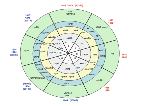
[See related figure below.]
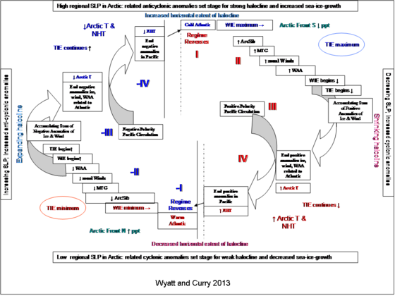
The stadium wave hypothesis - a hypothesis regarding multi-decadal variability of climate - involves interactive behavior within a network of ocean, ice, and atmospheric indices. The hypothesized network structure is such that a signal propagates sequentially through the network indices, with Eurasian Arctic sea ice being a critical link. As the propagation proceeds, regimes - multi-decadal intervals of warming alternating with intervals of cooling - evolve. Basically, on a multi-decadal timescale, a warming regime (mostly increasing NHT) is characterized by an increasing anomaly trend of AMO and the positive polarity of PDO anomalies; a cooling regime (mostly decreasing NHT) is characterized by a decreasing anomaly trend of AMO and the negative polarity of PDO anomalies. But how...
Variability of the stadium-wave signal is tied to the Atlantic. The AMOC (Atlantic sector of meridional overturning ocean circulation), via the AMO, is hypothesized to govern the tempo of stadium-wave propagation (WKT). The exact mechanism setting the pace for the AMOC is not fully resolved; hypotheses differ on whether the AMOC source is intrinsic, external, or a combination (see WKT and references within). But for the hypothesized stadium-wave signal, Eurasian Arctic sea ice appears to be the avenue by which the signal reaches beyond the Atlantic.
Unique to the Arctic Ocean is its Atlantic-sector juxtaposition to open ocean in winter. This proximity conveys dominant influence to the Atlantic on the feature most critical to Eurasian Arctic sea-ice growth in winter - the halocline. Thus, through the Arctic-Atlantic interface, sea ice extent in the Western Eurasian Arctic shelf seas varies in tandem with the AMO, and by extension, the AMOC. A cascade of positive feedbacks in the first stage of an evolving climate regime occur: changes in ice cover, SLP over the Arctic, in associated wind patterns and consequent sea-ice dynamics. Together, these changes amplify the Atlantic-born signal. In the background, seeds of gradual trend-reversal are embedded. Changing inventory of ice cover governs latitudinal position of the overlying Arctic Front, determining location of delivery of freshwater, upon which the halocline relies.
In the second stage of climate-regime evolution, positive feedbacks slowly are supplanted by negative ones, reversing the polarity Atlantic Ocean signal. Reasoning for this ties back to the halocline. A cold (warm) Atlantic promotes a strong (weak) halocline and increased (decreased) sea ice extent in the Western Eurasian seas in winter, which inhibits (allows) ocean-heat-flux to the overlying atmosphere, cooling (warming) the air at high latitudes, thereby increasing (decreasing) the polar-equatorial temperature gradient, which in turn, encourages (discourages) warm air advection from low latitudes poleward and eastward. Mid-and high latitude temperatures, especially over landmasses at lower altitudes, increase (decrease).
Positive feedbacks amplify the reversed-polarity signal during the third stage of regime evolution. Pacific involvement becomes evident in this stage. Sea-ice dynamics indirectly affect ocean-heat-flux via impacts on sea-ice cover, with opposing inventories between the Atlantic and Pacific sectors of the Eurasian Arctic. SLP over the Arctic is modified - largely a result of activity in the Atlantic sector. Also affected are the associated winds, the sea-ice-export patterns, the Atlantic influx into the Arctic, and ultimately, the Atlantic-based halocline. Simultaneously, modifications of the Arctic High are felt in the Pacific, the circulations of which positively correlate with the less dominant multi-decadal component of sea-ice growth in the Eastern Eurasian seas. Meanwhile, back in the Western Eurasian Arctic, the positive feedback cycle now in effect has re-drawn the halocline in such a way as to reinforce the dynamics dominantly in play.
The governing trend of NHT is most pronounced in the Arctic temperature. Changes here most strongly affect the multi-decadal component of the Northern Hemisphere's surface average temperature. As the fourth and final stage of climate-regime evolution engages, the entire hemisphere is now uniformly dominated by the NHT trend. Cumulative impacts of basin-scale winds, sea-ice changes and SLP modifications reinforce the prevailing Arctic and NH temperature trends. Both trends reach their most extreme values in this stage of regime evolution.
In the background, the Arctic Front, shifting in response to ice cover, negatively feeds back onto this mature regime. In addition, circulation patterns in and over the Pacific interact in such a way as to remotely and negatively feed back onto the Atlantic. Within a few years after the manifestation of maximum or minimum values of this multi-decadal temperature component in the Arctic and the Northern Hemisphere, the Atlantic circulation trend reverses. At this point, a new regime has begun.
Is the signal confined to the Northern Hemisphere's ocean-ice-atmospheric network?
The hypothesized stadium-wave signal, in the way described, propagates across the Northern Hemisphere through an envisioned ring-like network of ocean, ice, and atmospheric circulation patterns. It is doubtful that the network is confined to the North. Likely the Southern Hemisphere is linked through direct means in the Atlantic sector and indirect teleconnections related to the Indian and Pacific sectors, but this has not yet been studied. It is also doubtful that network interactions exclude the stratosphere, especially in light of the observation that the dynamics described above are pronounced in the winter, when the stratosphere couples with the troposphere through the polar vortex. In fact, recent studies (Schimanke et al. 2011; Omrani et al. 2013) suggest a link between the low-frequency winter signatures of: Atlantic SSTs, sudden-stratospheric-warmings (SSW), and modifications of atmospheric circulation in the troposphere over the North Atlantic - a dynamic that would be consistent with dynamics observed in stage two of regime evolution. But for now, this is speculation on my part.
Mann et al. 2014 have suggested that apparent signal propagation is a product of noise - i.e. due to a statistical artifact. Do they have a point?
On the Publications Page of this website, detailed responses addressing the points presented in Mann et al.'s paper are posted. They include:
1.) Two contrasting views of multidecadal variability in the 20th century (Kravtsov et al. 2014)
2.) "Is the stadium-wave propagation an illusion?" an essay by M. Wyatt summarizing Kravtsov et al. article (see above).
3.) "Disentangling Forced from Intrinsic Variability" an essay by M. Wyatt summarizing full reply to Mann et al. 2014 paper.
In short: Fundamentally differing views on the nature of how climate works underpin different analysis methods employed by Mann et al. and Wyatt et al. The different analysis methods generate different conclusions regarding the nature of signal propagation.
The Mann et al. work regarding low-frequency climate behavior is rooted in the assumption that behavior of all climate indices is dominated by a common, time-varying, externally forced (natural and anthropogenic) signal plus minor contributions from intrinsic interannual variability, represented by white noise.
In contrast, the hypothesis underpinning the stadium-wave is that on long-term time scales, the multi-decadal component of climate variability organizes into synchronized (matched rhythms, not necessarily same timing) network behavior, executed through coupled interactions of oceanic, ice, and atmospheric indices. This self-organizing, synchronized network behavior is ubiquitous throughout a variety of physical, biological, electrical, computer, and social systems.
Thus, it appears that these two views diverge into two camps: the low-frequency signal in climate is either forced or intrinsic. But, the reality is, things are not so simple.
A current focus in climate research is disentangling a presumed forced component (natural and anthropogenic) from a suspected intrinsic component. One school-of-thought asserts that observed time-varying behavior of the 20th century temperature record is mostly externally forced. This forcing derives from time-varying proportions of natural and anthropogenic contributions. The other school-of-thought interprets the secular-scale variability in the 20th century temperature trend as having a large intrinsic component - specifically, the multidecadal component. Many assume this component is tied to the multidecadal variability of the Atlantic Multidecadal Oscillation (AMO), and that the AMO is, in turn, driven by the Atlantic Meridional Overturning Circulation (AMOC). Both views - forced and intrinsic - hold merit. The argument regards proportion of contribution.
The stadium-wave hypothesis does not fall solidly into one camp or the other. Authors of the stadium wave propose that the stadium-wave propagation dynamic likely is intrinsic*, with the AMO as the pace-setter of the signal that propagates across the Northern Hemisphere on a multidecadal time scale through a network sequence of coupled ocean, ice, and atmospheric indices. But significantly, the stadium wave says nothing about the nature of the components of the AMO that generate its time scale of variability. The AMO variability may be externally forced, intrinsically generated, or a combination of both. The point is, the stadium-wave dynamic, on a multi-decadal time scale, is based on network behavior. Network behavior distinguishes itself by the observation that collective behavior is not the sum of behaviors of individual members. The network structure governs behavior. And in the stadium wave, collective interaction among network indices moves planetary heat - whatever its source - from one system to another, across the Northern Hemisphere, and likely with accompanying dynamics involving influence on ocean subsurface heat and dynamics of the stratosphere - topics for future investigation.
*at least with current boundary conditions - e.g. annually varying inventory of sea ice in West Eurasian Arctic, extant continental arrangement, orbital parameters of modern times, etc.
Closing thought:
This hypothesized signal is likely the result of many things, not the least of which are the existing boundary conditions that render the ocean-continental configurations and continental topography as they are, which, in turn, affect ocean circulation and wind patterns, directly and indirectly. The boundary conditions also govern oscillation times intrinsic to each ocean and allow for the existence of the 'global oceanic conveyor belt'. Self-organization properties, as discussed previously, allow for synchronized networks to grow, communicate, and increase in stability. Configuration of the network promotes propagation of the signal. How external factors, such as solar variability and anthropogenic forcing might affect the hypothesized 'wave' under current 20th century conditions has been discussed here; yet none of it resolved. Thus, assuming this hypothesized signal does indeed exist, and has in its current form for at least 150 years, and with modified amplitude and frequency for at least another 150 years before that, an appreciation for the elegance of this system is underscored. How comparable this might be to other climate periods -- where solar-insolation and distribution differ, or with different degrees of ice cover, as in the glacial periods, and further back, when ocean-continental boundary conditions differed -- is questionable; thus caution is used in extrapolation.